Hypersampled Model Predictive Control
Distinction between sampling and discretization
Access the paper here . Accepted to ACC 2024
Model Predictive Control (MPC) is a popular constrained control strategy for nonlinear systems. The idea behind MPC is to solve an Optimal Control Problem (OCP) at every instant and apply the first step of the optimal control sequence to the system. . Although MPC is widely used due to its stability, feasibility, and robustness properties (cite) , its widespread adoption is hindered by the fact that solving the optimal control problem in real time can be challenging. So we analyse the Hypersampled Model Predictive Control (HMPC) scheme, which is more efficient.
Introduction
Consider the continuous time system \(\dot x = f(x,u)\). The aim is to derive an optimal control law by solving the Optimal Control Problem (OCP), (Gautam & Nicotra, 2024) Equation 3. This can prove to be problematic, since this is an infinite dimensional problem. So, usual method of finding a control law is to discretise the system. This approach assumes that the dynamic model of the system matches the prediction model of the OCP.
An unfortunate consequence is that, for a fixed prediction horizon, reducing the sampling time inevitably leads to an increased number of prediction steps. This has the combined negative effect of increasing the numerical complexity of the OCP while also decreasing the allocated time for solving it.
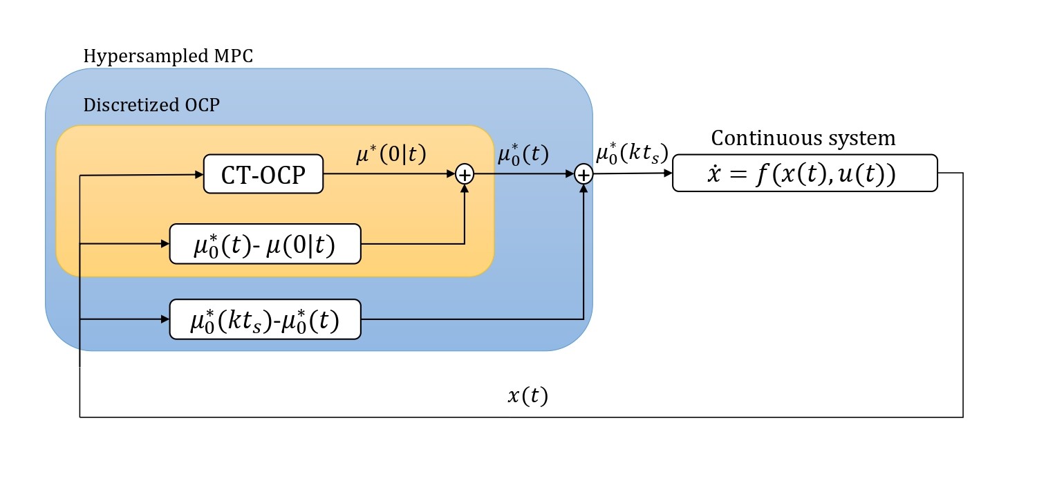
The paper seeks to formalize the distinction between discretization time \(t_d\), i.e., the step size used to discretize the continuous time system, and sampling time \(t_s\), i.e., the time at which the controller is implemented.
Experiments and Results
Numerical Experiments that validate the efficiency of the HMPC scheme were run on a point mass system and a Lane change problem. All levels of complexities have shown that the HMPC performs better than traditional MPC schemes.
We note the following properties: -Benefits of Decreasing \(t_s\): Reducing the sampling time tends to improve the performance of the controller by making it more reactive to external disturbances.
- Limit for Decreasing \(t_s\): Due to real-time imple- mentation requirements, \(t_s\) is lower-bounded by the computational time required to solve the OCP.
- Benefits of Increasing \(t_d\): Given a fixed prediction horizon \(T\) , a larger discretization time step leads to less prediction steps N . Since the computational com- plexity oscales with N , it is generally beneficial for td to be as large as possible. -Limit for Increasing \(t_d\): Since larger values of \(t_d\) increase the discrepancy between an upper bound on the maximal admissible error will translate into an upper bound on \(t_d\).
Point Mass System
The details of the Point mass system with disturbance can be found in (Gautam & Nicotra, 2024). We compare the performance of two MPC schemes and a HMPC scheme.
- MPC1: ts = td = 0.02s;
- HMPC: ts = 0.02s and td = 0.4s;
- MPC2: ts = td = 0.4s.
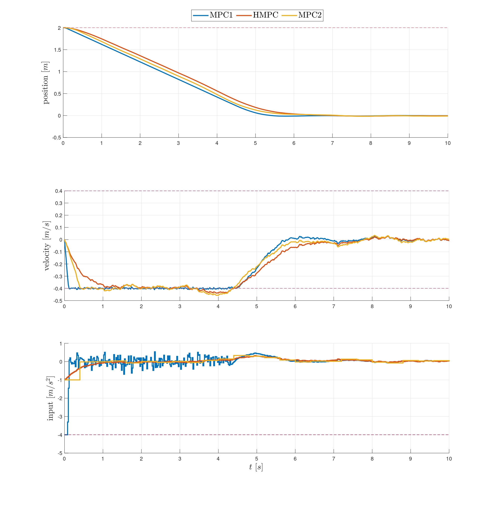
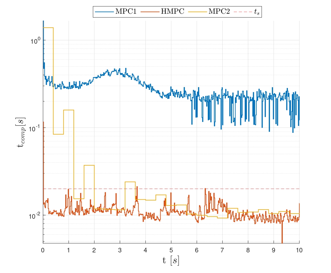
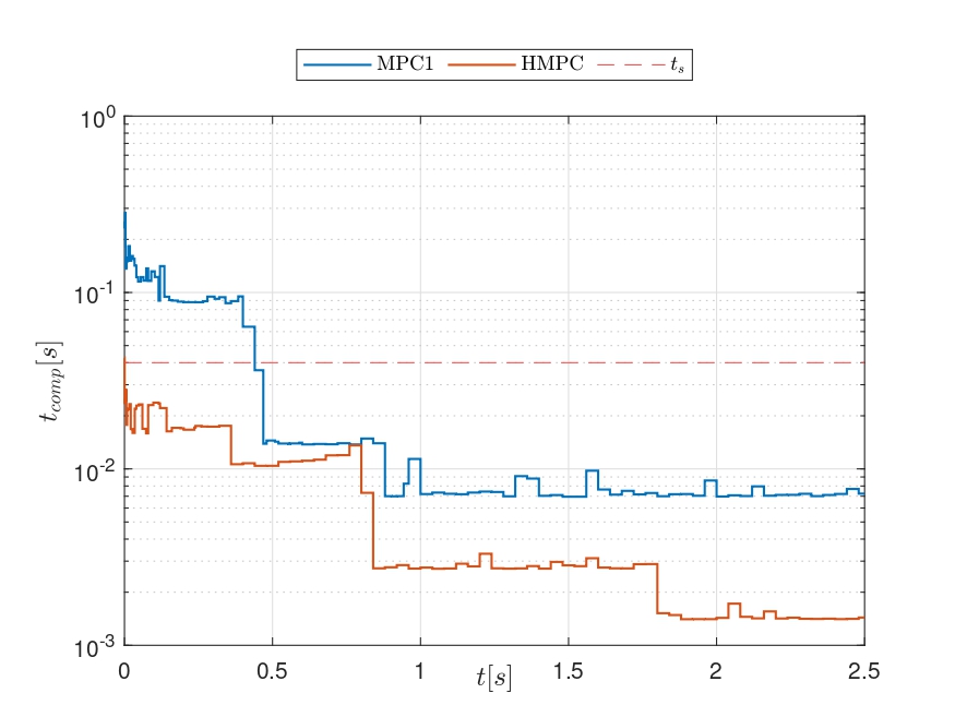
The disadvantage of MPC1 becomes apparent by examining the computation time required to solve the underlying OCP. As shown, the time required to solve MPC1 is approximately 30 times more than HMPC and MPC2. This is because MPC1 has a prediction length of N = 100 steps, whereas HMPC and MPC2 have a prediction length of only N = 5 steps.
Nonlinear Lane Change
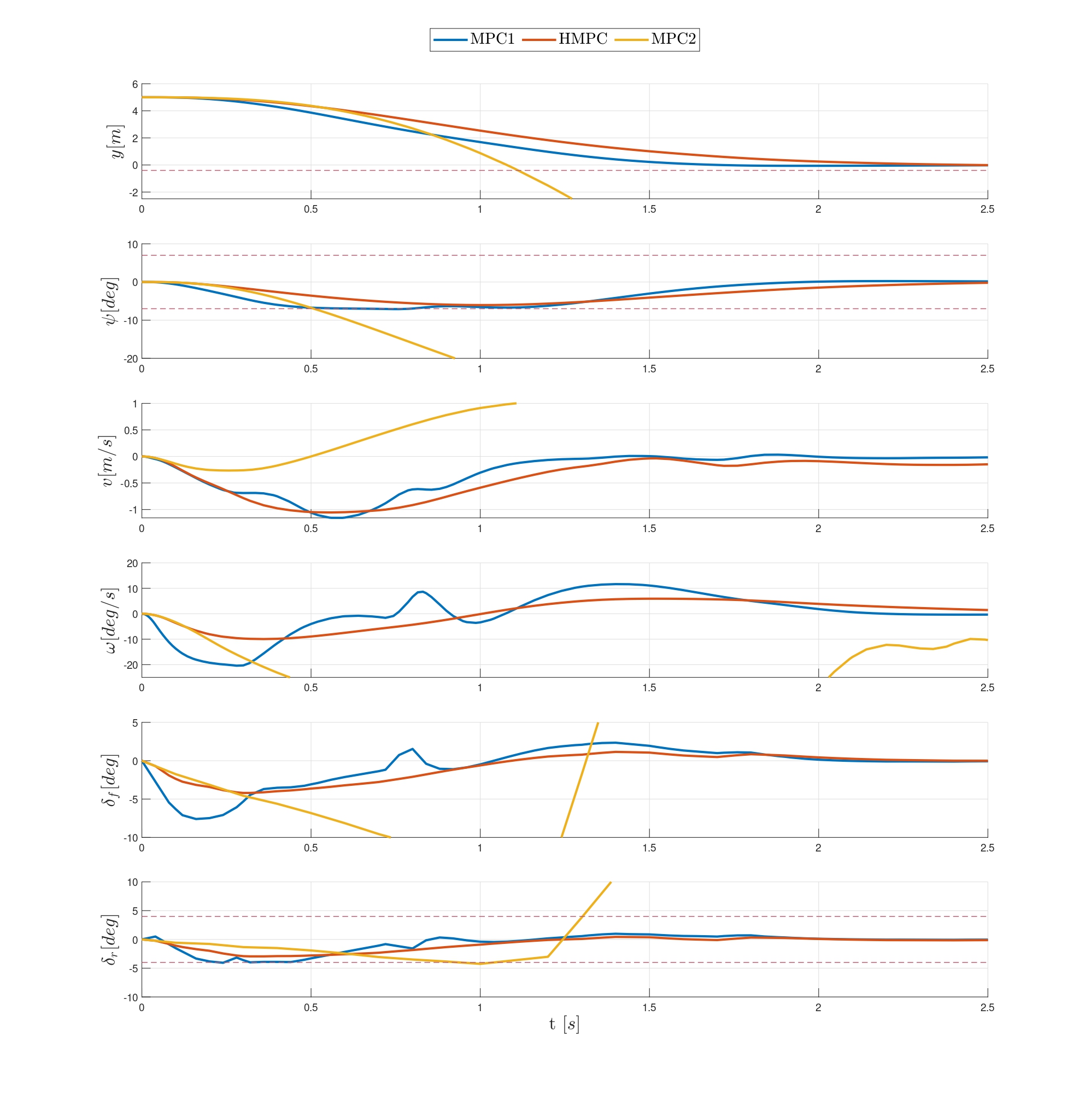
To emphasize the advantages of HMPC with a more complex example, we consider the nonlinear lane change system detailed in (Liao-McPherson et al., 2020). We compare the state and input trajectories obtained using three different schemes:
- MPC1: ts = td = 0.04s;
- HMPC: ts = 0.04s and td = 0.2s;
- MPC2: ts = td = 0.2s.
