Discretization Methods for Hypersampled MPC
Same performance, five times fewer optimization variables. Under review at ACC 2027
Under review at the American Control Conference (ACC) 2027.
S. A. Aravind, Y. Gautam, M. M. Nicotra. “Influence of Discretization Methods on Hypersampled Model Predictive Control.”
The problem
Standard discrete-time MPC ties three things together through one equation: the prediction horizon, the sampling time, and the number of optimization variables. Sample faster and the problem gets bigger while the time to solve it shrinks. That makes MPC hard to run on fast systems with limited onboard compute.
Hypersampled MPC (ACC 2024) broke that link by separating the controller’s sampling time from the discretization of the optimal control problem. This paper goes one step further: it drops the idea of a single “discretization time” altogether.
The idea
Instead of discretizing the system dynamics and then solving a discrete-time problem, we formulate the problem in continuous time and discretize its solution. Using input-to-state stability arguments, the paper shows that:
- the resulting MPC is asymptotically stable as long as the discretization is accurate enough, and
- it can be implemented as long as the sampling time is small enough.
The two conditions are independent, so accuracy and sampling rate can be chosen separately. And because stability depends only on how well the very first predicted input is approximated, the prediction steps don’t need to be evenly spaced. That opens up a new design space: put fine steps at the start of the horizon, where accuracy matters, and coarse steps later, where it doesn’t.
We compare three ways of spacing the prediction steps (fixed, modified fixed, and logarithmic), each with Forward Euler and 4th-order Runge-Kutta integration.
Results
The test case is an emergency lane change on a full nonlinear vehicle model with Pacejka tire forces. Each HMPC scheme uses N = 10 prediction steps, against a standard discrete-time MPC baseline with N = 50, all running at a 0.04 s sampling time. A standard discrete-time MPC with only 10 steps would need a 0.2 s sampling time, and that closed loop goes unstable.
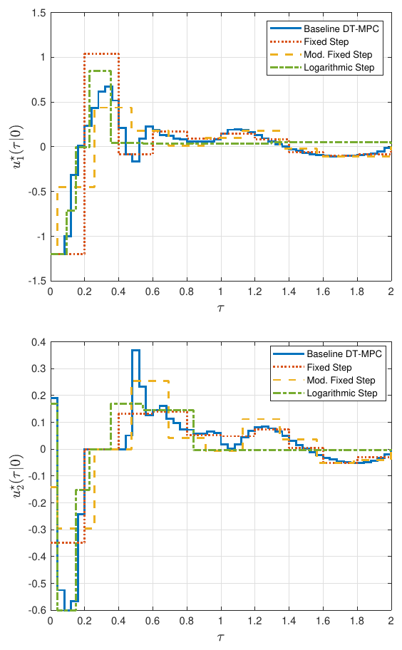
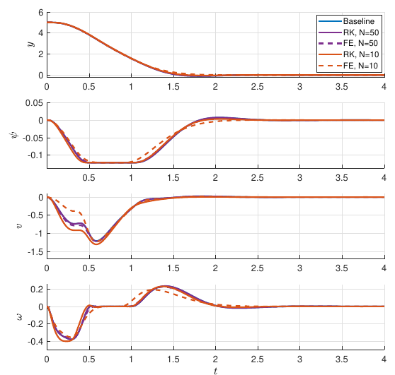
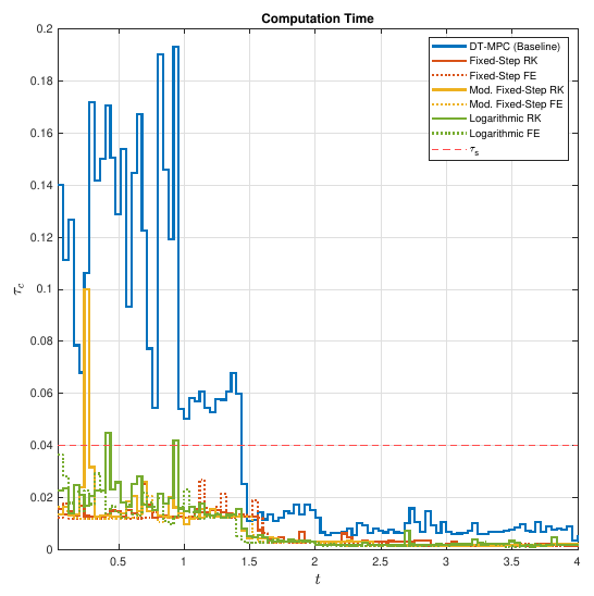
A counterintuitive result. Replacing Runge-Kutta with the less accurate Forward Euler makes predictions worse, but the closed loop becomes more damped, not unstable. A controller designed around an unstable integration scheme has to provide extra damping. As a result, Forward Euler stays stable as the number of steps drops, while Runge-Kutta goes unstable at N = 3. If an overdamped response is acceptable, the cheaper integrator can be the safer choice.